## Document Purpose This document is written to provide a detailed explanation of the methodology used to create Replica’s seasonal mobility model (Places). At Replica, we understand that data is valuable only to the extent that it is trusted to inform analysis and decision-making. To that end, this document provides an overview of Replica’s data sources, data processing methods, statistical inference systems, and data outputs, in order to help our customers evaluate the quality and accuracy of our models, and assess privacy and data security implications. ## Introduction Replica's seasonal mobility model (Places) is a high-fidelity activity-based travel model with network-link level granularity. Each model is a synthetically generated representation of the activities and movements of residents, visitors, and commercial vehicles on a typical weekday and typical weekend day for a given location and season. The output of each seasonal mobility model is a complete, disaggregate trip and population table. Each completed model also includes a Quality Report, which shows how the outputs of the model compare to ground truth data. The report facilitates comparisons and validations between Replica's modeled outputs and a customer's observed counts. Replica's seasonal mobility models are delivered at “megaregion” scale, most of which cover geographies that include between 10 million and 50 million residents. 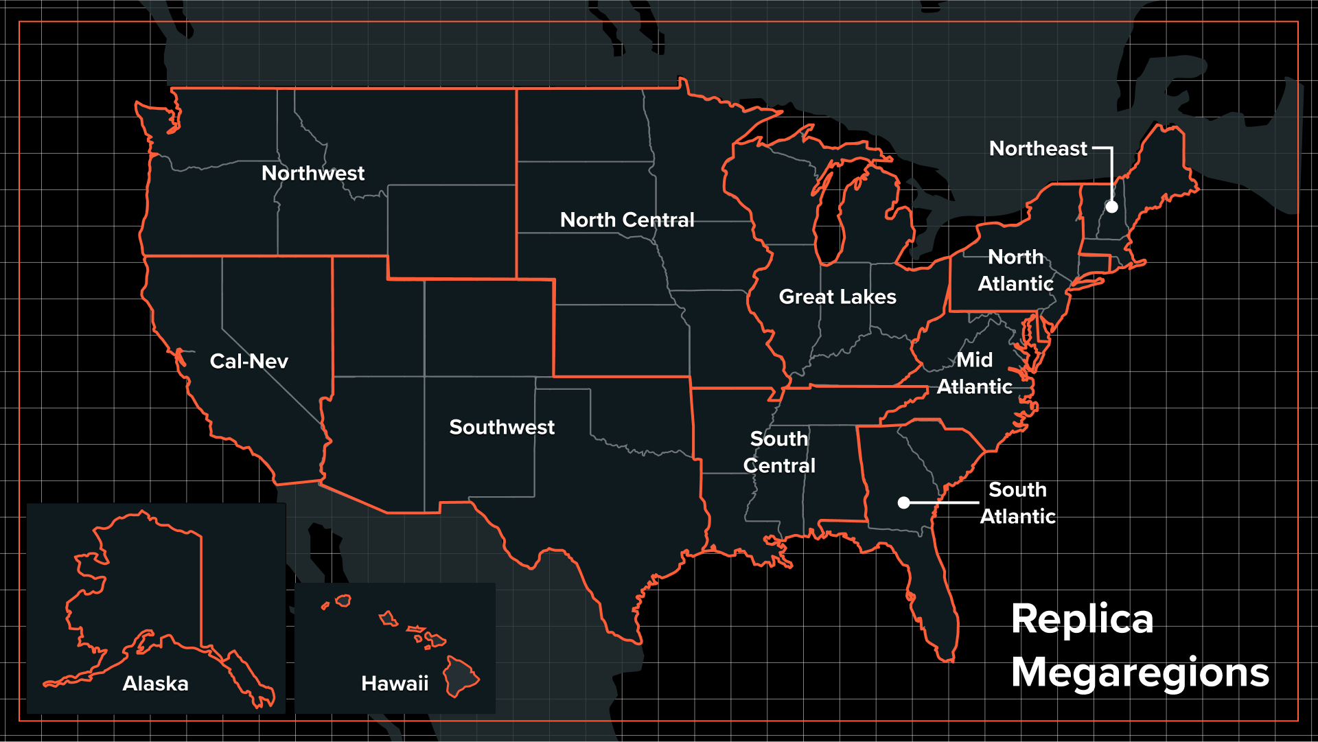Megaregion Boundaries

## Data Sources Replica's seasonal mobility model (Places) utilizes a diverse set of public and private data sources. This composite approach mitigates risk by minimizing sampling bias, creating resiliency against data quality issues, and protecting against data source disruption, while enabling Replica to deliver detailed modeled outputs. Building component models from different data sources independently also creates additional privacy protecting measures, as it enables Replica to abstract out potentially identifying details of any individual before combining these models into our aggregate outputs. These data sources fall into five broad categories: 1) Mobile Location Data, 2) Consumer / Resident Data, 3) Built Environment Data, 4) Economic Activity Data, 5) Ground Truth Data. This section provides a brief overview of each category of data. How each data source integrates into the data processing pipeline is addressed in later sections. ### Mobile Location Data Replica incorporates three types of mobile location data into its pipeline: 1) location-based services data, 2) vehicle in-dash GPS data, and 3) point-of-interest aggregates. Previous versions of Replica’s model also included cellular networks data as another source of mobile location data. _Location-based Services (LBS) Data_ As people move around with their phones in the real world, they use mobile apps that rely on their location, which is determined via GPS. Users opt in to sharing their location when using these apps. The user’s location as identified at a specific point in time is commonly referred to as a location trace. For users that opt in to sharing their location, mobile app publishers then aggregate these location traces, keeping the localization accuracy set at the device by the user. The mobile app publisher then de-identifies the traces and licenses them to data aggregators (e.g., Cuebiq, Safegraph, Gravy Analytics). Using the mobile advertising ID, or “ADID”, uniquely generated for each device, aggregators join data from multiple app publishers into a single-time sequenced data stream for each device. (Note: Users can reset their ADID at any time). A single data aggregator usually sees a sample size equal to approximately 10% of the US population. Because location traces are dependent on a device using a specific application, and recent Android and iOS operating systems are more and more restrictive in background location data collection, the space-time coverage of this type of data is often volatile. Replica sees data from more than 30 million unique devices each month. 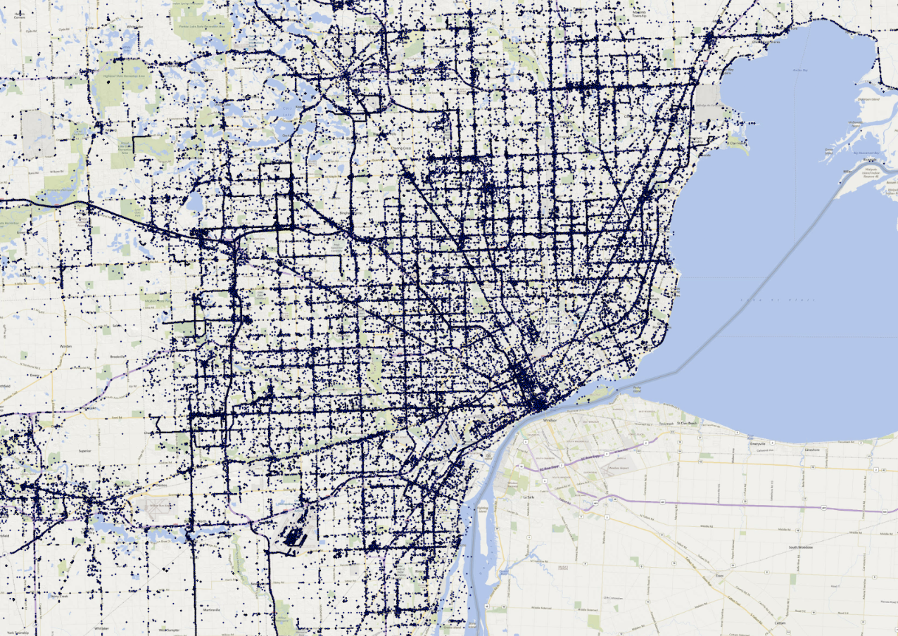Visual representation of raw location data collected from several thousand random devices for a period of 1 hour in the Detroit region, across all data types.

Visual representation of raw location data collected from several thousand random devices for a period of 1 hour in the Detroit region, across all data types.

_Vehicle in-dash GPS Data_ Car manufacturers often integrate both GPS and cellular connectivity hardware into their vehicles for real-time navigation, safety, and other services available through in-dash infotainment systems. This generates data on vehicle speeds and locations, which can be geo-matched to a particular road segment (telematics data), and transferred to centralized data storage and processing systems that monitor real-time congestion. The primary purpose of these systems is to provide better routing services to consumers and/or manage operations of specialized vehicle fleets (e.g., freight, shuttles, taxi vehicles). This telematics data is also licensed by third parties, which is governed by EULAs. Replica processes in-dash GPS data from over 3 billion trips each month. _Point-of Interest Aggregates_ Wireless technology can be used to detect and count an aggregate number of mobile devices present in a given venue (e.g., a park or a shopping mall). Aggregators of this point-of-interest (POI) information provide a total count of devices in their sample at each location, providing a signal to estimate the popularity of each venue. This signal enables Replica to generate the relative occupancy weights at different points and areas of interest for its own model. Replica processes POI data from over 4 million locations each month. ### Consumer / Resident Data Replica incorporates both public and private sources of resident and consumer data as the basis for creating a synthetic population. The majority of this data is sourced from the US Census Bureau. Replica utilizes the following US Census datasets: * [5-Year American Community Survey (ACS)](https://www.census.gov/programs-surveys/acs/news/data-releases.html) * [1- and 5-Year Public Use Microdata Sample (PUMS)](https://www.census.gov/programs-surveys/acs/microdata.html) * [Longitudinal Employer-Household Dynamics (LEHD)](https://lehd.ces.census.gov/data/) * [Census Transportation Planning Products (CTPP)](https://ctppdata.transportation.org/?utm_source=dlvr.it#/index) * [National Center for Education Statistics](https://nces.ed.gov/) * [US Department of Education](https://collegescorecard.ed.gov/data/) ### Built Environment Data Replica ingests and utilizes a number of sources for transportation network, land use, and real estate data. These include: * OpenStreetMap (OSM) * General Transit Feed Specification (GTFS) data. Replica updates its nationwide database of GTFS feeds twice each year. Currently, the database includes feeds for 440 agencies and 11,400 routes. If customers have GTFS data for additional agencies, Replica can add those agencies to its database. * A number of proprietary sources including providers of land use categorization data, parcel data, building footprint data, building floor area data, POI data (e.g., restaurants, stadiums, theaters), parking data, and hotel inventory data. Parcel-level data is collected for roughly two-thirds of the land area of the United States. ### Economic Activity Data Financial data processing companies collect and store the aggregate number and characteristics of transactions (such as dollars spent or the time of transaction) made at different categories of vendors within a given geography in a given period of time. This payments ecosystem data broadly has 3 sources: (1) Merchant Acquiring Data, which ties transaction data to the venue where the transaction occurred; (2) Bank Issuing Data; and (3) Payments Networks, which tie transaction data to the card making the transaction. Replica currently ingests 2 of those 3 sources of economic activity data. ### Ground Truth Data Replica uses a number of different sources of ground truth, or observed counts, to calibrate its models. This data is “held back” during the model creation phase and then used to calibrate initial outputs. Specific types of ground truth include, but are not limited to: * Auto / Traffic Counts, both in aggregate and for specific vehicle types (Private Auto, Freight) * Transit Ridership Counts * TNC/Taxi Counts Ground truth is both sourced by Replica directly, and optionally provided by Replica’s customers. Each of Replica’s seasonal mobility models can be sufficiently calibrated exclusively with Replica-sourced ground truth. The inclusion of customer-provided ground truth is neither a requirement nor a dependency to delivering a seasonal mobility model. Nor does the absence of customer-provided ground truth meaningfully impair the quality of a modeled season. However, certain customers with robust sets of ground truth data elect to include that data in the model calibration process to further calibrate the model, and to better compare Replica’s outputs against their own counts. 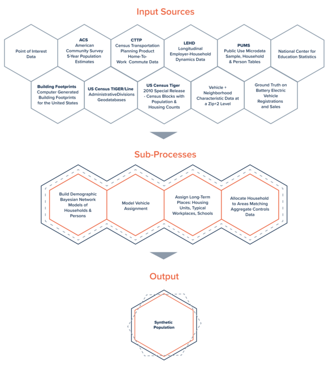## Core Data Product Creation The first step in the Replica seasonal mobility model (Places) development process is the transformation of source data into Core Data Products (CDPs). If the Data Sources described above are the “raw materials” to Replica’s development process, the four CDPs described below are the essential building blocks of Replica's model. A common characteristic of each CDP is that they produce nationwide outputs. ### Population CDP The Population CDP is a nationwide synthetic population that is statistically similar to the census population in person-level attributes, household composition, and in aggregate, at each census-level geography. These synthetic people and households are assigned to housing units, work locations, and school locations, which represent long-term choices that do not vary during the one-week simulated time period of an individual seasonal mobility model. Replica’s nationwide synthetic population is updated seasonally, using the following process. _1. Creation of Households and Persons_ The first step in creating the Population CDP is to train two Bayesian networks from the US Census’s Public Use Microdata (PUMS) sample files — one network representing households, and another representing person attributes. The purpose of the Bayesian network approach is to model a diversity of persons and households with attributes that reflect conditional probability distributions of the attributes specific to each given geographic area (e.g., a Public Use Micro Area [PUMA] in the US). In addition to geographical partitioning, the models are stratified by household size and person types: different household models are trained within each PUMA for households of a given size, and different person models are trained for a given role of a person in a household (e.g., employed adult, a child, a relative, etc). 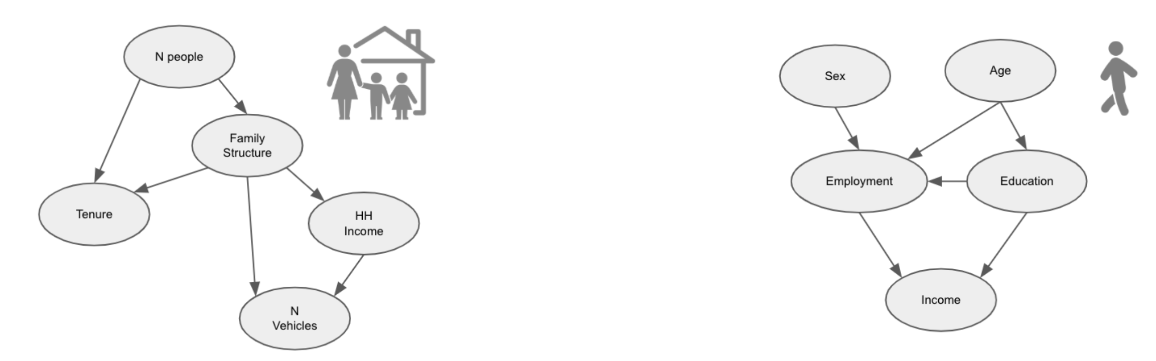An example of the Household and Person Bayesian network models structures.

An example of the Household and Person Bayesian network models structures.

The structure of the network represents conditional dependencies between the attributes. For example, for each household-sized group within a microdata sample area, for a particular household of a given size belonging to a given household-income group, the Bayesian network includes a link that represents the probabilities of owning different numbers of vehicles. Sample structures of the models are shown in the figure above. When data is available, the set of standard attributes and the structure of the Bayesian network model can be extended, learned from data, and customized to include other variables of interest as well as to integrate auxiliary and proprietary data sources required for a particular use case. _2. Matching Controls in Aggregate_ In the second step of building the synthetic population, the system allocates microdata-based household profiles to census areas, (typically block groups), in order to match the known total census aggregate numbers (i.e. “controls”), using a convex optimization method. The output of the optimization method is a set of weights which, for every census area, describe how many times a given set of controlled seed attributes of a given household and person's record should be used for a matching Bayesian network model to generate a synthetic household and persons. Not every person or household attribute can be “controlled” for in this method, so only salient attributes are chosen. These attributes, which are used as a set of controlled variables, include: household size, household income group, the number of vehicles owned, employment status, industry of employment, commute mode, housing tenure, age group, sex, race, ethnicity, and school grade attending. Meta-controls at the PUMA level are included in the allocation algorithm’s objective function. Due to the internal inconsistencies in census aggregates (attributed to data suppression, binning thresholds, and non-sampling errors), limited accuracy of data for hard-to-reach populations, presence of significant special population groups in given areas (e.g., military establishments), and other reasons, the allocation algorithm parameters may require adjustments considering the robustness of the synthesis with respect to data versus the overall accuracy across different areas. At the end of this step, households and persons are generated by passing each household’s profile and their members through the Bayesian network developed in the first step. In addition to the controlled seed attributes, each person and household is assigned other attributes based on the relationships and probabilities of the Bayesian network models. 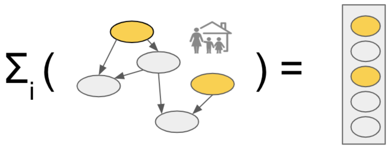The purpose of the allocation step is to find a combination of the households (weights) to use as seeds in Bayesian network synthesis, such that the total set of synthesized households and persons in aggregate match the given “controls” for the main attributes of interest within each area.

The purpose of the allocation step is to find a combination of the households (weights) to use as seeds in Bayesian network synthesis, such that the total set of synthesized households and persons in aggregate match the given “controls” for the main attributes of interest within each area.

_3. Home, Work, and School Assignments_ In the final step of the process, households are assigned to housing units within a census block group, and employed persons and students are assigned workplaces and schools, respectively. Home, work and school assignments are made at the sub-census block group resolution for the purposes of modeling fidelity and are not exposed in Replica’s user interface. * _Housing._ Decennial census estimates of the total population and dwelling units available within each census block, as well as proprietary or customer-supplied land use, geocoded postal addresses, and building footprint data are used at this step to improve spatial fidelity and modeling realism. While it is possible to adjust the controls and update the synthetic population to reflect recent population changes not captured by census, or to reproduce future scenarios, a standard Replica release is generally based on the most recent 5-year ACS data. * _Places of Work._ Each employed synthetic person is allocated first to a workplace at the census tract-level, then at the census block group-level, then to an individual office unit. Using a combination of the most recent Census Transportation Planning Product (CTPP) tabulation of the ACS data and location-based data used to generate weekly home-work assignments, we construct a home-work matrix representing the number of residents traveling between a home census tract to a work census tract based on their commute mode, industry of employment and income group. The reason for incorporating the home-work allocation into the home-work assignment is to see seasonal changes in work assignment since CTPP data is generated infrequently and the most recent CTPP data was from 2016. These flows are given as marginal distributions in CTPP, and an optimization algorithm is applied to reconstruct the conditional distribution of the workplace as a function of the employed person’s attributes. Land use and LEHD employment data are then used to redistribute flows to census block groups within tracts, according to the availability of employment in any given industry sector. Once work block groups have been assigned to each employed person, the individual office unit assignment leverages parcel land use, building, points of interest, and industry information to identify the most likely work location for that person. * _School Enrollment._ School-aged residents are assigned to a school location based on each school’s enrollment, school district boundaries, and proximity to home. Students are assigned to schools that offer classes matching their ages. Grade levels and enrollment counts are sourced from the US National Center for Education Statistics for the relevant school year. Residents aged 16 (legal working age) to 18 are assigned to a secondary school until enrollment counts are met. The balance of these residents will assume their general employment class (e.g., not in the labor force, employed, or unemployed). Residents aged 18 to 23 and 23 to 34 are assigned to undergraduate and graduate institutions respectively using the same process, until total enrollment counts are met. Residents who are classified as employed and a student are considered to have part-time employment and may attend school and a workplace on the same day. _4. Vehicle Assignment Modeling_ In the Spring 2023 season, Replica introduced vehicle assignments. Each private auto trip is now tied to one of two vehicle fuel types, Battery Electric Vehicle (BEV), or vehicle with another fuel type. Vehicle assignment is modeled as a four stage process: * _Model the marginal attributes with respect to vehicle ownership for each household_. Data from a consumer marketing vendor is used to understand the temporal and spatial variability of different vehicle ownership attributes. This vendor collects data from a variety of sources including self-reported survey information, property data, and vehicle title/registration documents. We use two datasets at the zip+2 granularity: 1) a set of characteristics of the vehicles owned within the households of a given zip+2, and 2) sociodemographic characteristics of the individuals and households in the zip+2. We combine these datasets to produce a dataset at the zip+2 granularity that includes automotive and sociodemographic characteristics. For example the percentage of households that own a Battery Electric Vehicle (BEV), average household income for the zip+2, and percent of households by age distribution. We run a K-Nearest Neighbor algorithm taking into account the sociodemographic attributes of Age and Household Income using this combined zip+2-level dataset, and the previously synthesized households. As a result, every household in our synthesized population is assigned a set of average household characteristics, including the percent of households that own a BEV. * _Model the target number of electric vehicles that exist in each zip code_. Our data vendor provides an estimate for the total number of vehicles, and the percent of households that own an electric vehicle in each zip code. However, the total population of vehicles may differ between our synthesized population and our data vendor. For states where we have publicly available data on BEV registrations or BEV sales, we normalize the zip code level vendor data to match state totals. We then produce a target number of BEVs for each zip code. * _Generate the set of synthetic vehicles for each household._ Once all households have been assigned the most likely average vehicle ownership characteristics, and all zip codes have a target value for electric vehicles (N), we sample N households using a weighted sampling with replacement out of the set of households in that zip code. The weight used is the percentage of households that own a registered electric vehicle, a property that was assigned to each household in the first step. Thus, the sociodemographic characteristics of households that are more likely to own a BEV are captured. * _Assign the vehicles in the household to individuals._ We assume that the same individual uses the same vehicle throughout the day. In cases where a household has more individuals above driving age than vehicles, the same vehicle can be assigned to multiple people. After a vehicle is assigned to an individual, we assume that individual uses that vehicle for every private auto trip on the modeled day.

In addition to the resident synthetic population, Replica generates a population of visitors for each modeled megaregion. Visitors are sampled from the nationwide synthetic population and anchored to visitor-relevant locations: lodging facilities (e.g., hotels) and ports of entry (e.g., airports, border crossings). Visitor counts are scaled using a composite of data sources, including hotel occupancy and entry-point throughput. ### Built Environment CDP The Built Environment CDP consists of a number of distinct data tables. The primary data output of the Built Environment CDP is a nationwide land use model that serves as the source of truth for all spatial data consumed by Replica’s systems. It maintains three principal layers of disaggregate data: (1) parcels, or “lots”, (2) buildings, and (3) points of interest. The union of these three layers with auxiliary spatial datasets such as schools and airports supports the home, work, and school assignments in the Population CDP, and the location choice model for activities in Replica's seasonal and weekly mobility models. It is responsible for creating the comprehensive set of locations an agent can travel to. The land use of buildings and parcels is classified using direct input data from proprietary sources where available, and otherwise modeled using tract-level characteristics. Parcel-level data can come in a variety of forms, including spatially joined points of interest, zoning descriptions, and postal delivery codes. Tract-level characteristics consist of aggregate land use proportions that are further weighted using the relative, block-level concentration of housing units in Census data. Replica’s hierarchical land use categories are as follows:

Primary category (L1)	Sub-categories (L2)
residential	single_family multi_family
commercial	retail office non_retail_attraction
mixed_use	* combination of an other L2s
industrial	industrial
civic_institutional	healthcare education civic_institutional
transportation_utilities	transportation_utilities
agriculture	agriculture
open_space	open_space
other	other
unknown	unknown

Total square footage for each building is modeled using a composite of individual and aggregate features. Dwelling units are modeled on each residential or mixed-use parcel based on ACS-scaled Census counts. Points of interest are classified based on North American Industry Classification System (NAICS) industry code. The Built Environment CDP also includes a number of distinct datasets that serve as “base layers,” such as the OSM network and nationwide GTFS. All datasets are refreshed seasonally. ### Economic Activity CDP The Economic Activity CDP is a weekly estimate of total consumer spend across a number of categories, for every census tract in the country. An estimate is created for both (1) all “brick and mortar” spend, defined as the sum total of every transaction that occurs in-person within a given tract, regardless of where the purchaser lives, and (2) all on- and off-line resident spend, defined as the sum total of all transactions made by residents of a given tract, regardless of where that transaction occurs. Consumer spend includes all transactions, including credit card, debit card, and cash transactions, that take place at a point of sale, such as at retail stores, supermarkets, restaurants, taxis, and bars. It also includes e-commerce transactions in these same categories. The data does not include all household expenditures; for example, rent, car payments, and healthcare spending is excluded. This most closely aligns Replica's consumer spend metric to the Census Bureau's Monthly Retail Trade Estimates. Transactions are categorized by the merchant’s NAICS code. Both Brick and Mortar and Resident Spend for each census tract is generated for the 6 categories listed below. Due to source data limitations, an on- and off-line breakdown for Resident Spend are only generated for three of the six categories, which are marked with an asterisk. 1. Restaurants & Bars* 2. Retail* 3. Grocery Stores* 4. Airline, Hospitality & Car Rental 5. Entertainment & Recreation 6. Gas Stations, Parking, Taxis, & Tolls Outputs are generated based on three types of source data: (1) Cardholder transaction data; (2) Merchant transaction data; (3) Point of Interest visitor patterns data. Outputs are calibrated against multiple sources of ground truth, including both Census and Bureau of Economic Analysis (BEA) datasets. At a high level, the methodology consists of 3 steps: (i) aggregated spend by home location (both in-person and e-commerce); (ii) disaggregate spend by POI and aggregated spend by merchant location; (iii) updated in-person spend by home location using disaggregate estimator. First, we use vendor data (which consists of transactions at merchants and for individual cardholders) to estimate the total spend (in-person + e-commerce) and use the cardholder data to determine what proportion of the total spend is e-commerce. According to census totals, we capture about 10-20% of total transactions (depending on the category), and to estimate aggregate totals, we scale up based on the population within each home tract. To correct for sample bias, we combine nationwide monthly census totals and state-wide annual totals from the BEA to a forecasted state-wide monthly estimator that forecasts ahead to the most recent month. We then scale up tract-level totals using state-wide bias correction factors based on the previous 12 months (to ensure the modeled spend is always forward-looking). Scaling factors typically vary from 1-3x depending on the state and category. Second, we model POI-level spend using a combination of merchant-level transaction data and POI-level visit count data. Our POI-level model includes visit count data, transaction data, population data, and POI-specific features such as name, common brands, etc. We scale up POI-level spend to ensure consistency with aggregate totals generated in the previous step. Scaling factors are done at the PUMA level since PUMAs have relatively consistent populations. Finally, to improve the spend-by-home location estimator (for in-person spend only) we use our POI-level spend estimator from the previous step in combination with POI-level modeling of home tract using POI-level visit count data. ### Travel Activity CDP The Travel Activity CDP is a nationwide set of travel behavior models — “Personas” — that describe and predict the movements of individual residents. These travel behavior models are trained using a combination of the mobile location data acquired by Replica as described earlier. The purpose of creating personas from observed travel behaviors of real people is three-fold: preserve privacy of source data, provide explanation for travel behavior, and enable model sensitivity to urban design and policy changes. The personas are composed of three main underlying behavioral choice models: activity scheduling, destination location, and travel mode, which will be discussed in detail below. A combination of these models can be used to reproduce complete daily activity sequences (e.g., start the day at home, drive to work, walk to lunch at lunch break, complete work, drive to shop, shop, drive to home, stay at home) with each activity annotated with planned start and end times. _Staypoint Creation_ The first step in the creation of the Travel Activity CDP is the transformation of traces to staypoints and travel periods. For each device identified by a non-persistent hash of device ID, individual location points (traces) are clustered with a space-time clustering method in order to identify recurrent locations where the device has been stationary over a period of time (a staypoint). The time gap between two consecutive staypoints is labeled as a period of missing data or, in the presence of consistent intermediate locations, a period of travel. The location of each stationary activity is assigned a ”staypoint ID” specific to that device. This process runs daily. Staypoints are analyzed seasonally (Spring, for instance, includes March, April and May data). For each season, the set of staypoint IDs for a given device is referred to as the device user’s “habitat.” Repeated activity locations are annotated with a common staypoint ID, which is used to identify repeatedly visited locations. A combination of land use attributes (generated from the Built Environment CDP) and an observed recurrent pattern of stay at the most frequented locations is used to identify home and work locations of a device owner. Home and work activities are identified in the sequence of device movements along with their typical start/end times and durations. Home and work (if observed) are the two most prominent activity types. Following the assignment of home and work activities, a combination of land use, popularity scores for a set of venues at a given time, and the context of the stay time period within the sequence of the primary activities within the day are used to assign likely activity types to all secondary staypoints. The figure below illustrates the three location data and main processing stages: 2) raw location data, b) staypoints detection and activity types inference, and c) travel periods segmentation and mode inference. 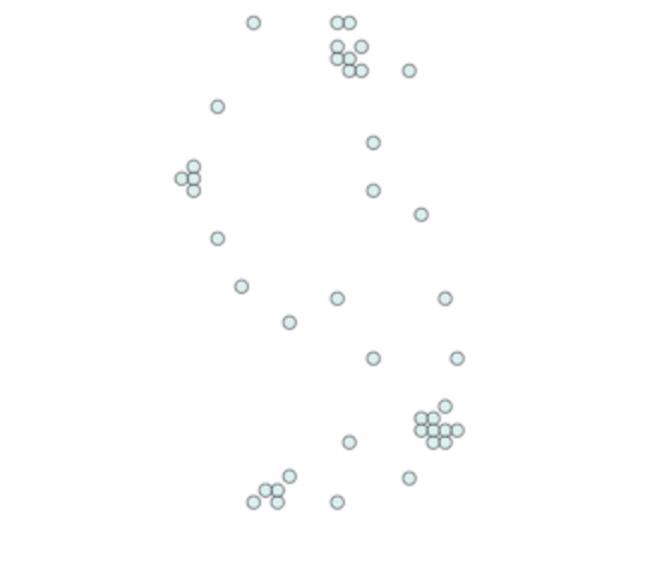a) Raw location data

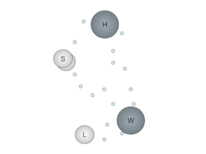
b) Staypoints detection and activity types inference

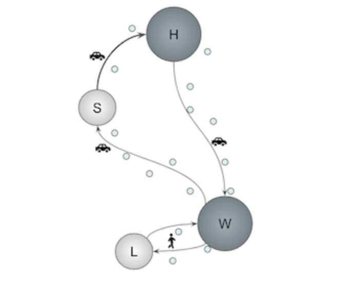
c) Travel periods segmentation and mode inference

_Known Limitations in Staypoint Detection_ During the staypoint creation process, insufficient spatial accuracy or a high dispersion of locations within individual clusters may lead Replica to deem the data not usable. At each stage in the process, data can be withdrawn from further processing in the pipeline depending on the quality and accuracy of the previous stage. For instance, when significant temporal gaps are present and the coverage is not sufficient to identify secondary staypoints, the data from a device may only be useful to inform algorithms that require aggregate information of home and work flows. It is worth noting that the start and end time of any activity (and the arrival and departure time for each travel period) cannot be observed with certainty in LBS and cellular data. A typical duration of a period of stay that can be detected from a typical mobile location data feed with continuous temporal sampling (1 location sample per minute) is a stay of over 5 minutes in duration (over 85% detection accuracy), with most stays of 15 minutes identified at 90% accuracy. Very short activities or local activities that happen within the range of localization accuracy can not be reliably detected. For example, it is often not possible to identify events such as buying a coffee at a drive-through location, particularly with no significant stationary periods (such as a long wait in line). _Generating Personas_ Models of travel behavior (“personas”) of adult residents are trained using mobile location data that was successfully processed into segmented sequences of staypoints and periods of travel as described above. Records from devices with insufficient temporal coverage or insufficient number of complete day records are not used for model training. A complete day is defined as a day with at least 14 hours of coverage (last observed time minus first observed time) and no gaps of more than three hours. Devices with fewer than 7 days of observed overnight stays during each season at identified home locations are also removed from the training data set. Assigning attributes — such as age group, income, and employment status — to each persona is required for travel modeling (as well as the assignment of personas to the synthetic population). **Because Replica does not acquire nor handle any personally identified information (PII) associated with device owners, these attributes are inferred** using (1) the demographics of the residents and workers for the given home census block group; and (2) the socio-demographics of the workers with a given home-work commute pair detected for a persona as compared to that provided by the most recent CTPP. Commute mode detection and the presence of recurrent home-based trips by car gives a proxy for a vehicle availability attribute. Weighting factors are computed based on the total number and the number of employed persona models residing within a given census block group. Iterative proportional fitting methods used in weighting traditional surveys are applied for the latter. These weighting factors are in turn used in the adjustments of home-to-work commute flows and persona matching. Three models are trained for each device: (1) Activity Sequence Model (ASM), (2) Travel Destination Location Choice Model (LCM), and (3) Mode Choice Model (MCM). Each model is described below with respect to how the model is structured and trained on the observed data, including the privacy protection measures applied in the process. _(1) Activity Sequence Model (ASM)_ The annotated “activity day sequences” (staypoints and travel periods) form the basis of the device persona’s activity sequence model. ASM is a generative sequence learning model. When given historical data on the observed sequence of activities, it can produce the most likely sequence of activities of a person carrying the device on a given day of the week within the season. ASM is also used to fill in short unobserved gaps and predict the likely sequence of activities at the end of the day given its observed beginning. Three hour gaps in the observed data are imputed with the activities predicted by the ASM. This gap-filling functionality of the ASM includes access to a complete library of activities detected with high confidence and shared across all the devices observed in the region. Without mitigations, activity sequences carry a privacy risk: A person could be re-identified if they have a rare or unique activity sequence that is reproduced in the synthetic data. Specifically, in the event a rare activity sequence is reconstituted in the modeled outputs (e.g., gym visit at 5 am every Wednesday followed by visiting a specific restaurant), it is possible to regenerate a part of a real person’s rare day itinerary. To mitigate this risk, we filter out rare day sequences from the training dataset. Rare or unique sequences are identified by resampling it at regular time intervals within a 24-hour period beginning at 03:00 local time, and comparing across all observed activities. Figure 5.5 gives an example of this representation (using 30 minute resampling interval) for several days, where each row represents a day with the actual calendar date and day-of-week as metadata. 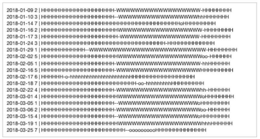Example encoded day activity sequences for a single device/user (H:home, W:work, o:other, '-':in transit, h: secondary home).

Example encoded day activity sequences for a single device/user (H:home, W:work, o:other, '-':in transit, h: secondary home).

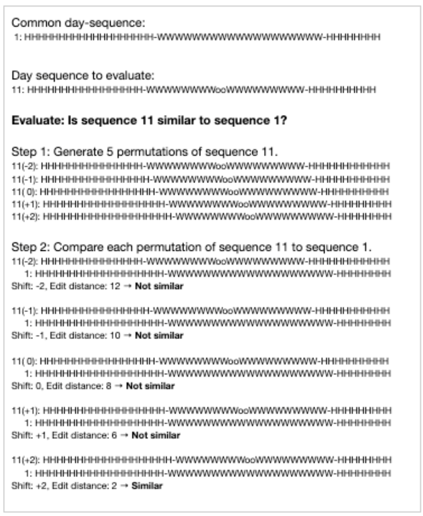
Two day-sequences are considered similar if there is less than one hour shift in either direction and have less than two 30-minute time bins with different activity types. The figure below provides a working example. The “rare” day-sequences are then compared against each of the common day-sequences. If they are similar, the sequence is kept, otherwise it is removed from the dataset. Working example of similarity between two day sequences.

Working example of similarity between two day sequences.

At least 20 similar activity sequences have to be observed across all devices in order for a given sequence to be included into both a training set and the common library used for gap filling. Elimination of rare day sequences generally results in a lower trip rate than initially observed, an unavoidable consequence needed for privacy protection. _(2) Location Choice Model (LCM)_ The location choice model is trained per device to learn and predict travel destination location choices for discretionary activities (i.e., not home/work/school) made by the device owner. The LCM operates at a disaggregate level, selecting individual privately-owned businesses (e.g, individual businesses, shops, services) and other venues (e.g., parks, places of historic interest, tourist attractions) as potential destinations. It is a model that, for a given set of alternative destinations represented as attributes of particular venues in the area, ranks them based on the observed choice made by the owner of the device, considering every other location ever visited by a person as an alternative. Every trip made for a discretionary activity observed becomes one training sample for the LCM for a given person. The LCM includes contextual variables such as distance to home, distance to work, a score describing the deviation from a regular home-work commute, the hour of the day, day of the week, allocated travel time, and duration of the next scheduled activity. For destinations located in dense commercial and urban areas when an exact venue visited by a device cannot be observed, the training sample is constructed from a combined set of attributes (using the same contextual variables and median values of accessibility variables). _(3) Mode Choice Model (MCM)_ The mode choice model consists of two distinct components. The first is a mode inference model that assigns a likelihood score to each mode that could be used for every observed trip. It is a discriminative machine learning model with a strong prior based on geographical location of origin and destination, accessibility, and observed travel times and distances. It is often impossible to distinguish the mode from the observed attributes of a trip, particularly in dense urban areas with significant congestion, where a pattern of biking, taking a bus, riding in a taxi, or driving a private vehicle could have the same speed profile. The mode inference model is additionally conditioned on the context of the trip within a day (e.g., which tour the trip is a part of and what modes are not feasible), as well as the pattern of modes taken on recurrent trips for the same origin and destination, such as daily commute to work. Modes that are detected with high confidence are considered to be revealed preferences and serve as the inputs for the next stage. The second component is a mode choice model that gives the likelihood of choosing a given mode, as a function of the alternatives and the inferred attributes of the decision maker. Given an origin and a destination with respective start and end travel times, routes are computed for each possible mode (private auto, walking, bicycling, public transit with different access/egress types, and on demand auto) and are included into a choice set for a given trip. Choice model structure is based on machine learning with a utility function specification that includes a standard set of attributes (travel time, cost, in-vehicle and out-of-vehicle times, walking duration, inferred age and household income, vehicle ownership) and an additive alternative specific constant (ASC). _Special Cases in the Travel Activity CDP_ Since Replica does not acquire mobile location data for minors, children and students are represented with a simplified model. Residents below the age of 5 do not receive a persona. All their travel is assumed to be represented by the travel of an accompanying adult from the household. K-12 student personas are constructed synthetically, with the only daily activity being a trip to school. College student personas can represent students who are partly employed, and attend school and work on the same day. College student personas also have variability in class start and end times. ## Model Creation To create an individual seasonal mobility (Places) model, the CDPs are used to produce a simulation of a typical day of all movement in the modeled megaregion and season, leveraging the observed data in an accurate and privacy-preserving way. This synthetic representation is created using a 3-step process: (1) Persona Matching; (2) Activity Generation; (3) Mobility Simulation, each of which is described in detail below. 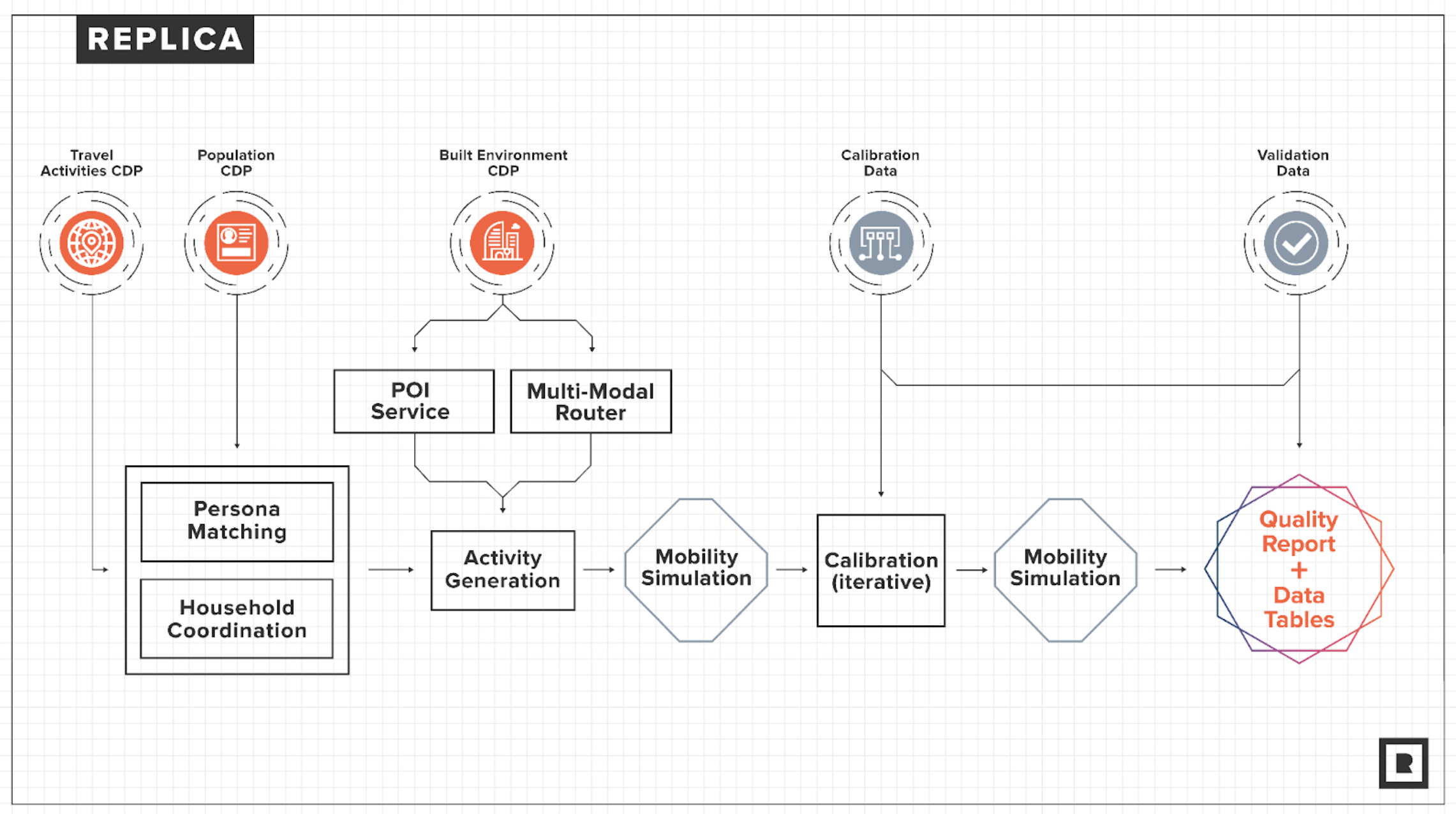Model creation diagram

Following the 3-step process, the synthetic representation is calibrated and validated to observed travel metrics relevant to the given day of the modeled season. The calibration process is described in the later sections. ### Persona Matching The first step in the model creation process is to “motivate” a synthetic person to travel by matching that resident with a persona. For a given model, each synthetic person that “lives” within the megaregion boundaries is matched with a persona from the same geographic area and season — in essence, joining the Population and Travel Activity CDPs. Residents aged 18 and older are matched with either working or non-working personas, depending on their employment status. A working synthetic resident is matched to a working persona that closely matches its home and work locations. Alternatively, a non-working resident is matched to a non-working persona that is found near its home location. This is done by weighting the personas using their inferred night-time locations as compared to the residential population (all persons aged over 7 years not living in group quarters) given by the ACS 5-year estimates. Iterative proportional fitting methods are used for reweighting, following a methodology similar to those used in household travel surveys. Personas from areas with a lower device coverage are weighted higher than ones from areas with higher coverage. Candidate personas are then ranked by a weighted combination of the proximity of their home and work locations and, for working personas, the alignment of the persona's typical work-departure time with the local work-departure-time distribution from the American Community Survey. The top 25-50 matches based on the proximity score (with exact limit randomly chosen each time) are returned. A persona is then chosen at random from the resulting set. School-aged residents (5-18) and college students are matched with a special student persona. Persona matching is performed sequentially for all members of the household. Generally, for each specific megaregion and season, the expected ratio of adult residents to available personas is approximately 8:1. That is, if a megaregion has a synthetic population of 20 million adults, there would be approximately 2.5 million potential personas. Visitors are matched to visitor-specific personas - distinct from resident personas - and included in both the Activity Generation and Mobility Simulation steps alongside the resident population. ### Activity Generation Following the joining of synthetic persons and personas, the activity sequence model, location choice model, and mode choice models are each applied to generate activity. The activity sequence model is applied at the beginning of the simulated typical day, assuming the day starts at home for all residents. Location choice and mode choice models are sequentially applied for each tour and a trip of the simulated day. _Generation of Activity Sequence Model (ASM)_ First, the ASM returns day sequences sampled from the trained model. ASM is applied sequentially for all the adult members of the household. For employed adults in the households it includes deterministic coordination of the morning commute in terms of departure times and escorting a student to school. For school-aged students, an age-dependent fraction travels via carpool — highest for elementary-age children and declining through high school — to reflect parent drop-off patterns. The remaining school trips go through standard mode choice, including walking, biking, transit, and private auto, when the student is of driving age. It is at this point in the model creation process that a work-from-home determination is made for each employed adult in the model. Whether or not an employed adult commutes to work or works from home on the modeled day is determined using a composite model that factors in industry of employment, home location, and the aggregate behavior of device personas that share the same home Census Public Use Microdata Area (PUMA) during the modeled season. A typical trip rate produced by the standard version of an ASM is 3.7 trips (4.7 activities) per person per day for the nationwide sample of composite LBS/cellular data. This number varies geographically depending on the region, community type, and other factors. Region-specific trip rates are available in each megaregion’s Quality Report. _Generation of Location Choice Model (LCM)_ Locations of primary activities (home, work and school) are assigned at the population synthesis stage and are not chosen within the simulated day. For every discretionary trip, the LCM is queried with the synthetic person’s current (in simulation time) day-of-week, time-of-day, distance-from-home, distance-from-work, and commute deviation scores to rank accessible destinations for the planned activity type. The highest-ranked location is predicted by the LCM, but is not selected directly. Instead, it is used as a center of a spatial query to a POI service, which itself utilizes the Built Environment and Economic Activity CDPs. The POI service returns between 10 and 25 nearby venues of the matching category (exact count is randomly chosen). Every venue in the vicinity of a location returned as a candidate destination has an assigned popularity score computed from a combination of POI visits and credit transactions data, specific to the day of the week and the hour of the day when a visit takes place. Laplacian noise of variance, which is a function of a persona’s total number of observed visits in a day, is added to the raw place visit counts before this popularity score is computed. From this return set, a single venue is sampled based on the weighted popularity score (which may or may not be the original POI predicted by the LCM) and is assigned as a travel destination. _Generation of Mode Choice Model (MCM)_ Following the assignment of a travel destination, the mode choice model is applied at the tour and trip level, generating an array of available route options between the current origin and the planned destination, based on the state of the transportation network at that time. The set of routes include an available set of transit options (utilizing all relevant agencies from Replica’s GTFS database) as well as multiple driving routes, with the travel times accounting for the expected congestion along each alternative. Commute mode choice is governed by a separate model specifically trained on commute trips as described above. Tactical choices of modes for the trips within the tours are restricted based on the availability of a private vehicle (both car and bicycle) on the tour. It is assumed that a personal vehicle is accessible from any other destination accessed by walking from the last destination accessed by vehicle. General parking availability and capacity at activity destinations are not enforced in the current version of the model. Park-and-ride lots are an exception: lot-level capacity is tracked during simulation, with lots that have reached capacity excluded from the candidate set when assigning park-and-ride trips. ### Mobility Simulation Representation of all travel in the region on a typical day is derived with an agent-based simulation approach where every synthetic person in a household is engaged in travel to perform the activities at locations and times as predicted by their respective persona models. Interactions within the realized travel itineraries such as traffic congestion are accounted for in simulation runtime as described below. _Traffic Assignment_ Routing algorithms in Replica use a combination of the observed routes from mobile location data and observed link-level speed collected from in-dash GPS, and a version of dynamic traffic assignment using link-level representation of congestion (traffic state is assumed to be the same along the link). Vehicle trips are assigned to the network incrementally for each vehicle, with subsequent drivers departing earlier or later than originally planned and/or rerouting in response to the developing congestion in the bottlenecks. Routing is performed on the OpenStreetMap network which is algorithmically verified for the consistency of attributes (number of lanes and speed limits) and is processed for ensuring routability. Observed traffic volumes and routes are used in the network attributes verification process by ensuring the road types, number of lanes, speed limits, and turn restriction attributes are consistent with the traffic volumes observed on a typical day in a given season. No simplifications are applied to the network in terms of the categories of the roadways available for traffic, walking, and cycling. Route choice and link performance functions are data-driven, and informed by the routes and travel speeds as observed in the in-dash GPS probe data. For instance, the true vehicular capacity of road segments is estimated replicating the Highway Capacity Manual speed/flow approach for every major road in the country that reaches capacity within the data available. These capacities are fed into the link performance functions and used to make re-routing decisions as the simulation progresses and congestion builds up. The observed state of the network for a typical day is used for initial route planning, and the state of traffic on the network is stored for all the links and is updated in simulation time. The modes that interact in congested traffic are all vehicular modes (e.g., private autos, TNCs, and commercial vehicles) with the exception of public transit vehicles. All drivers are assumed to be completely and equally informed of the state of the congestion and having access to the same routing service returning multiple distinct route alternatives per route choice request. Vehicle trips start and end at a road link adjacent to the destination, as opposed to, for example, a parking lot or a parking structure nearby. In contrast, real drivers tend to circle for parking, miss turns, and drive between different entrances of large destination areas such as the multi-lot parking areas at shopping plazas. In reality, drivers may take a non-optimal exit from the parking lot, make a U-turn, or any number of unusual actions that are not represented in routing vehicles in simulation. _Transit_ Transit routing is based on the regional transit system represented by the set of the General Transit Feed Specification (GTFS) schedules valid during the simulated season in the modeled megaregion. The complete set of GTFS data used in a given season are available for download for reproducibility. In simulation, transit stops can be accessed by walking, biking, carpooling and private auto over the same network as other motorized and non-motorized movements. Egress modes include walking, carpool, on-demand auto and private auto. Park and ride (P&R) behavior is implemented in the current version of Replica. Transit route options that include an ingress leg of private auto are considered when modeling inbound commute tours. These alternative routes are only added for those transit stations with available parking. The new alternatives are then included as part of the set of options returned by the router. The transit router returns multiple options for every trip given the departure time window of 15 minutes from the planned departure time. Transit route choice is implemented as a machine learning-based model that includes walking distance, waiting time, number of transfers, in-vehicle travel time, and an estimated fare as attributes for every alternative. Additive constants representing idiosyncratic route preferences can be adjusted in calibration. _On-demand Auto (Taxi and TNC)_ On-demand auto is one of the available modes in the option set. Mobile location data alone does not allow reliable identification of trips made by an on-demand auto (vs. for example a carpool). The choice of an on-demand option is usually a function of the limited option set of modes available to reach the observed destination on the tour/trip, with lack of access to a personal vehicle. It is preferable to use auxiliary ground truth data sources to represent travel by taxi and TNCs more accurately. On-demand auto trips with a passenger are a part of the traffic flow that contribute to congestion. _Non-motorized Travel_ Non-motorized travel (walking and biking) is represented on the same street network as auto travel. Walking speeds are assumed constant; cycling speeds vary with road grade — slower on climbs, faster on moderate descents, and capped at walking speed on extreme slopes. Routing for both modes uses a generalized cost rather than pure travel time: pedestrians prefer direct routes on main roads, and cyclists additionally prefer routes on bike-friendly or car-free infrastructure and avoid steep climbs. Travel speeds are assumed constant and do not vary by characteristics of travelers (e.g., age) or network (e.g., width of sidewalks), with travel time as the objective function in shortest path algorithms. Origins and destinations of travel are set as the centroids of the building footprint traveled to/from, and the travel is considered started/completed from/at the travel link that is adjacent to this centroid. The accuracy of the representation of non-motorised travel is prone to the completeness and accuracy of the network, errors in the network attributes, as well as idiosyncratic route choices made by the travelers that might not be observable or representable due to the data limitations. At this time, Replica also only includes purposeful non-motorized travel in its model. Recreational trips (such as jogging for a workout, or a walk around a neighborhood or park that starts and ends at home) are not included. _Commercial (Freight) Travel_ Commercial vehicle traffic is represented in the simulation and outputs of the model. Commercial fleets of medium and heavy vehicles are modeled by using a different statistical weighting methodology; while freight vehicles contribute to congestion, their travel is not subject to rerouting due to behavioral response to expected delays. _Pass-Through Traffic_ Pass-through traffic is represented in the simulation and outputs of the model. Pass through (external-to-external) trips are a weighted sample of the devices that travel through the simulated region. The weighting methodology is similar to the one used in persona weighting and is aimed to represent the variability of the spatial coverage of the mobile location data sample. Carpool formation in the vehicles of pass-through traffic is not modeled and the occupancy rate is assumed fixed at 1.5 persons/vehicle. Routes of pass-through travel closely follow empirically observed routes (assuming they are the revealed route preferences in response to congestion). One reason Replica produces models at megaregion scale is to minimize the amount of pass-through traffic. ## Model Calibration and Quality Reporting After each individual simulation run, the modeled outputs are compared to aggregate control group data (i.e., observed counts, or “ground truth”) for quality and reporting purposes. This calibration process involves solving a set of large-scale optimization problems with an objective function defined as “fit to observed ground truth.” A careful balance is struck to ensure that the calibration algorithms do not overfit the modeled outputs to the calibration data, as both outliers and a certain level of noise is often present in every dataset. Each completed seasonal mobility model includes an associated Quality Report that displays a comparison of modeled outputs to ground truth data, enabling users to compare model outputs to observed counts. Customers have the option to supplement this process with their own ground truth data. However, it is important to note that the inclusion of customer-provided ground truth for calibration is neither a requirement nor a dependency to delivering a seasonal mobility model. Nor does the absence of customer-provided ground truth meaningfully impair the quality of a modeled season. ### The Calibration Process The calibration process compares modeled itineraries and the resulting travel volumes to observed counts, incorporating all ground truth available for the specific megaregion and season. Traffic data, transit data, and non-motorized travel data can all be incorporated into the calibration process. Data collected from induction loop sensors, toll gantries, computer vision, turnstile and ticket sales, tap in/out systems, as well as manual counts, can be used. _Data Verification and Processing_ The first step in the calibration process is to verify all data for consistency, identify the presence of gaps and outliers, and process the data to represent a typical day of the week in the modeled season. For example, average traffic volumes/ridership over all Wednesdays within a season are used to represent a typical Wednesday. Data outliers are identified and removed both algorithmically and manually in the cases of significant uncertainties. When day-specific information is not available, a typical weekday and weekend information is compiled in a similar manner. Replica can process a wide range of ground truth. For traffic flow calibration, hourly volumes are preferred but not required. Per-zone trip volumes (origin-side and destination-side, by hour and tract) can be used to calibrate per-zone adjustment coefficients in the utility function — currently applied to on-demand auto choice. For transit calibration, Replica aims to use the total number of boardings (ridership) per individual transit line. When little ground truth is available in a specific region, an estimation of trip volumes by a direct demand model trained on ground truth in other regions can be substituted. Calibration algorithms are particularly sensitive to ground truth data quality. Every sample introduced into the calibration system is validated for the feasibility of its data. Faulty sensors, which might throw off the calibration accuracy, are identified and removed in a cascade of algorithmic data quality and feasibility filters. For example, in the figure below, there’s an outlier in the upper-left data point where the modeled count is significantly higher than the field count. The expanded upper-left diagram shows a significant day-to-day variance, which indicates this sensor is unreliable and should not be used. 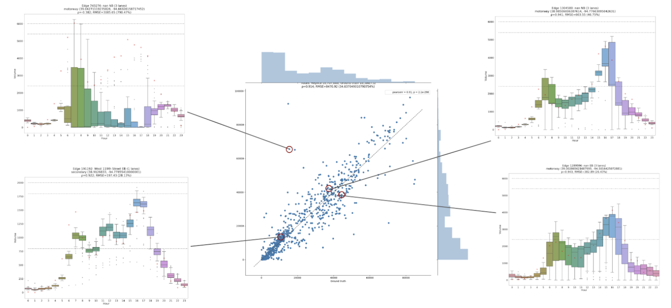Example traffic count calibration scatter plot (center graphic) for an hour window. The X-axis is field count; the y-axis is modeled count. Inlet diagrams represent hourly volumes in a 24-hour period with an empirical variance and outliers presented as box plots at each hourly bin.

Example traffic count calibration scatter plot (center graphic) for an hour window. The X-axis is field count; the y-axis is modeled count. Inlet diagrams represent hourly volumes in a 24-hour period with an empirical variance and outliers presented as box plots at each hourly bin.

_Running Calibration_ Once all the faulty counts are removed from the calibration set, the calibration process is run. Choice parameters are adjusted in the calibration process depending on the ground truth data availability. They include route choice preference constants (i.e., tendency to choose a longer route with less experienced delay due to recurrent congestion), carpool choice preference, transit route choice parameters as a function of transit type and particular transit lines in an available transit option (i.e., light rail might be more attractive than a similar bus option), and TNC choice parameters (as a function of observed TNC zone-to-zone trip volumes). In the calibration process, the algorithms are controlled to not overfit the calibration data. Despite the best attempts at validating ground truth data consistency and accuracy, both outliers and a certain level of noise are often present in every dataset. There is a delicate balance between the accurate fit to the ground truth data and the internal consistency of the simulation. There are often cases where the algorithms accept significant differences in certain counts if the modeled data represents a more consistent and balanced system state across other related metrics. These differences are typically resolved in favor of the model consistency and the observed data artifacts are disclosed to the customer. 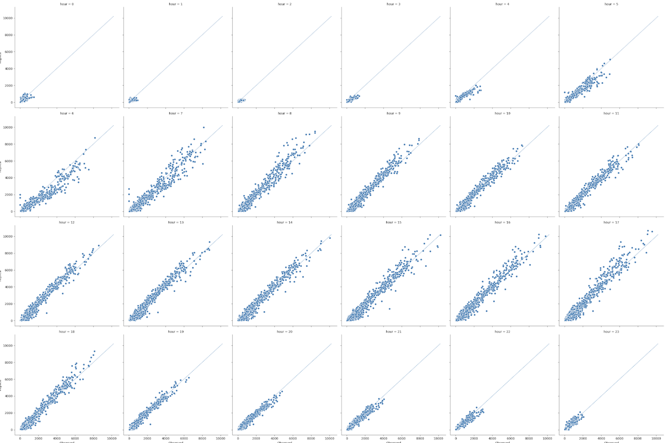Simulated hourly traffic volumes as compared to ground truth over a course of 24h period.

Simulated hourly traffic volumes as compared to ground truth over a course of 24h period.

### Quality Reporting The final step in the seasonal mobility model deployment process is the production of a Quality Report, which both summarizes the outputs of the model and compares the modeled outputs to Replica-sourced and customer-provided ground truth. In the spirit of transparency and measurability, Quality Reports are always made available to Replica customers for each available season. The Quality Report for each megaregion / season combination includes two types of information. The first is summary statistics, such as trip rate (both overall and by specific cohorts), mode and purpose breakdowns, and transit ridership counts. The second is a comparison of modeled outputs to ground truth. Root Mean Square Error (RMSE) is calculated, and plots and tables are provided in the Quality Report, for a number of key metrics including: * Commute departures by county * Auto volumes by hour and by road volume * Transit ridership by transit mode, transit agency ridership, individual transit agencies, and by route * Taxi/On-Demand volumes by origin & destination PUMA Quality Reports for each megaregion are available in our Help Center [here](http://help.replicahq.com/en/collections/1606964-quality-reports). Example reports can be made available to prospects by request. ## Data Outputs The methodology detailed above outlines Replica’s approach to running large-scale, computationally intensive simulations. It is this approach that enables Replica to deliver granular data outputs that match behavior in aggregate, but don’t surface the actual movements (or compromise the privacy) of any one individual. As such, the output of each simulation is a complete, disaggregate trip and population table for an average weekday and average weekend day in the modeled season (e.g., Fall 2021). The model represents a 24-hour period with second-by-second temporal resolution, and point-of-interest-level spatial resolution. Each row of data in the simulation output reflects a single trip, with characteristics about both the trip (e.g, origin, destination, mode, purpose, routing, duration) and trip taker (e.g., age, race/ethnicity, income, home location, work location). The disaggregate nature of the data means that data can be filtered, and cross tabulated, by characteristics of either the trip or trip taker (or both). Specifically, the seasonal mobility model development process results in the generation of two specific output tables: * [People Table](doc:demographics-employment) * [Trip Table](doc:disaggregate-trip-tables) Data from these tables can be joined using Person ID.