
[Discontinued] Weekly Economic Model Methodology
Due to changes in upstream data sources, this data no longer meets Replica's standards for reliability, and we have discontinued Spend data as of December 28th, 2024.
Methodology
Summary
Replica's weekly economic model combines publicly available data and vendor data to produce three customer-facing tables: Weekly Spend (by home location), Weekly Spend (by merchant location), and Weekly Spend County-to-County Flows.
The publicly available data sources used are:
- US Census Advance Monthly Retail Trade Survey - released monthly, but on a 3-4 month lag to reality.
- US Census Quarterly E-Commerce Report - released monthly, but on a 3-4 month lag to reality.
- Bureau of Economic Analysis Consumer Spending by State- updated annually, around October with the previous year's data
- American Community Survey 5-Year Population Estimates
The vendor data sources used are:
- Merchant transaction data: All in-person credit and debit card transactions for a subset of merchants. This data includes 60-70 million transactions per day.
- Cardholder transaction data: All credit and debit card transactions for a subset of cards issued, including both in-person and e-commerce transactions. This data includes 8-10 million transactions per day.
- Visit counts: Foot traffic data for a large set of merchants/points of interest. This data includes approximately 3 million stores where spending activity occurs.
These data sources are then used for modeling and calibration. First we create synthetic ground truth, and estimate spend by home geography and spend per merchant. Then, we calibrate home spend and merchant spend. Read about these steps in more detail below.
Detailed Methodology
There are 5 main steps in the weekly economic model. Below, a diagram shows each of these steps.
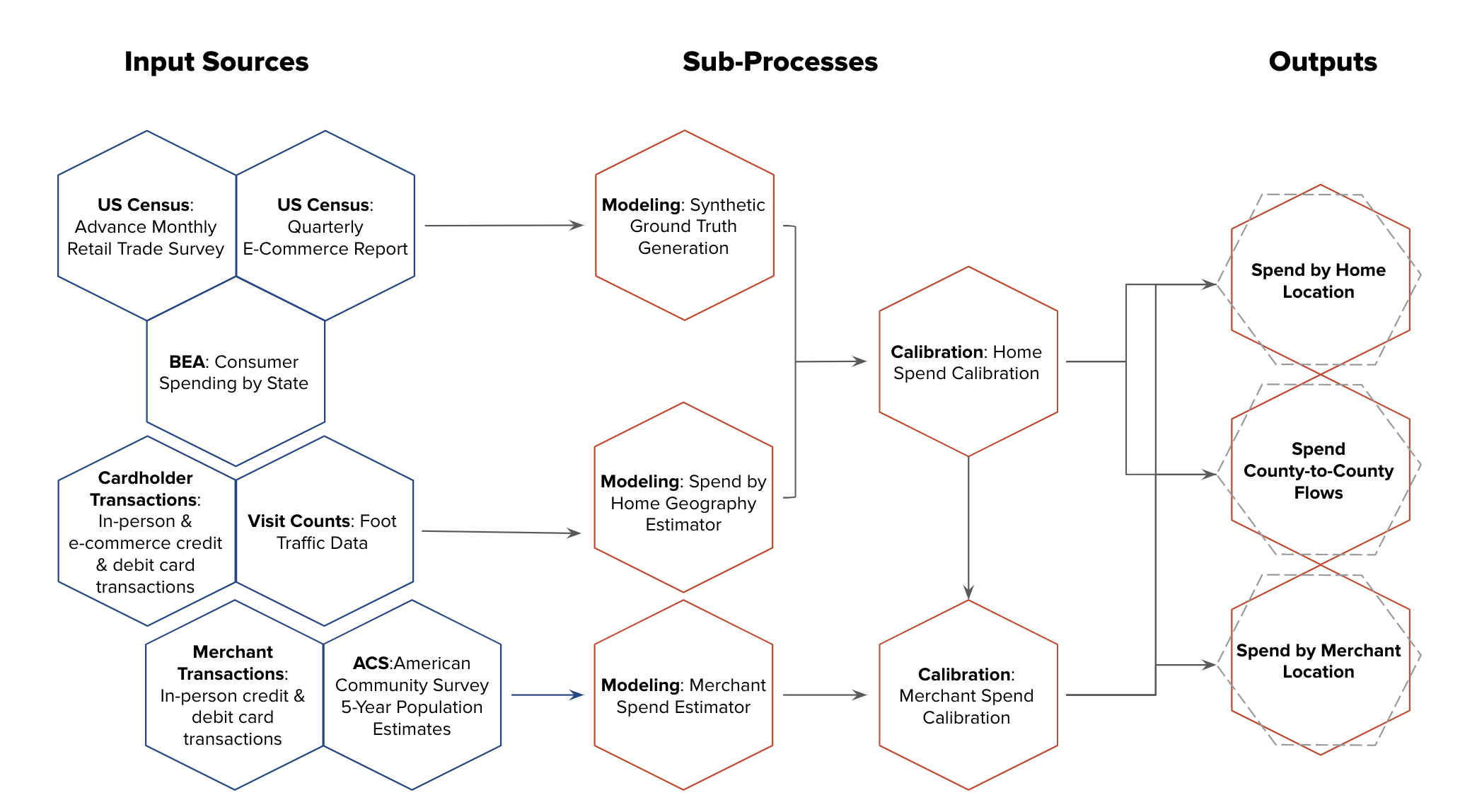
1. Synthetic ground truth generation
The publicly available Ground Truth sources we use are US Census bureau retail sales (both total and e-commerce) and Bureau of Economic Analysis (BEA) consumer spend tables. The census totals are provided at a nationwide-monthly cadence for total sales, and a quarterly cadence for e-commerce sales. However, they are typically 3-4 months behind the current date. On the other hand, BEA typically releases state-wide annual totals for a year during the following October.
To create up-to-date “synthetic” statewide monthly totals, we first forecast nationwide monthly totals using an auto-regressive time-series model. The model uses the latest 3 months of Census bureau data available, and use features for the forecasted months in previous years to account for seasonality. Then, we use the latest state-wide annual totals from the BEA to apportion the forecasted nationwide monthly spend by state.
2. Spend by home geography estimator
In the spend by home geography estimator, we use the cardholder transactions dataset that includes both in-person and e-commerce transactions on a subset of cards. Since we only receive a subset of cardholders across the USA at any given point in time (about 10-15M), we first estimate spend per person and then use population data to scale that to a total spend per tract. For example, suppose we have cardholder data for 30 people in a tract and the total population is of the tract is 3000. We would then scale spend in the tract by 100. With this approach, we assume that spending behavior is relatively consistent within each tract.
Then, we aggregate this estimator to the PUMA granularity, ensuring sufficient quality given relatively low sample size.
3. Merchant spend estimator
The merchant transactions dataset includes many more transactions (60-70M per date) but only includes a subset of merchants. On the other hand, we have visit count/foot traffic data from an extremely large (approximately comprehensive) set of merchants/POIs. To take advantage of this we use a semi-supervised regression model where we predict the spend per visit for each merchant/POI where the labelled data includes the merchants/POIs in our merchant transactions data, and the unlabelled data includes all merchants/POIs not in our transactions data but in our points of interest data. We then run a standard regression model where the features include population features for the geography of the merchant and merchant features such as name, major brands, e.t.c. This generates a spend per visit estimate for each merchant/POI. To calculate total spend, we multiply the spend per visit by number of visits from the visits source data.
4. Home spend calibration
In computing Spend by Home Geography, there is bias as cardholders included in the panel are not a random selection. To correct for this bias, we use the statewide monthly synthetic ground truth to compute scaling factors based on the previous 12 months of data. More concretely, we add up the last 12 months from the synthetic ground truth and the last 12 months from the home geography estimator and take a ratio to compute the scaling factor. The scaling factor depends on the industry but is typically in the range of 1-5.
5. Merchant spend calibration
Finally, to account for biases in the data, we again compute a scaling factor for each PUMA based on the in-person spend from the calibrated home spend estimator. Hence the total spend for each merchant/POI is scaled up to ensure that the in-person spend totals from the calibrated home spend data are met. This also helps account for non-credit card transactions.
Final Output
These modeling and calibration steps produce two tables: (1) Spend by home location, including in-person and e-commerce transactions, by tract, and (2) In-person spend per merchant and home tract. These two tables are used to create the three customer-facing tables Spend by Home Location, Spend by Merchant Location, and Spend County-to-County Flows.
Validation
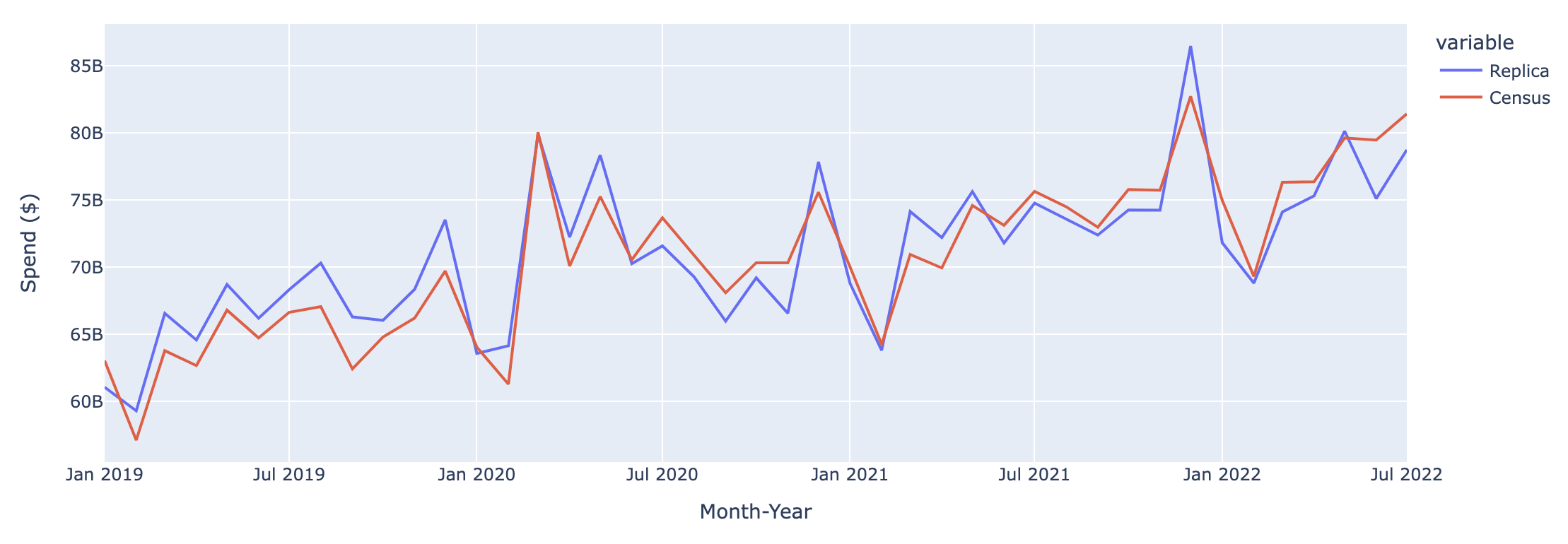
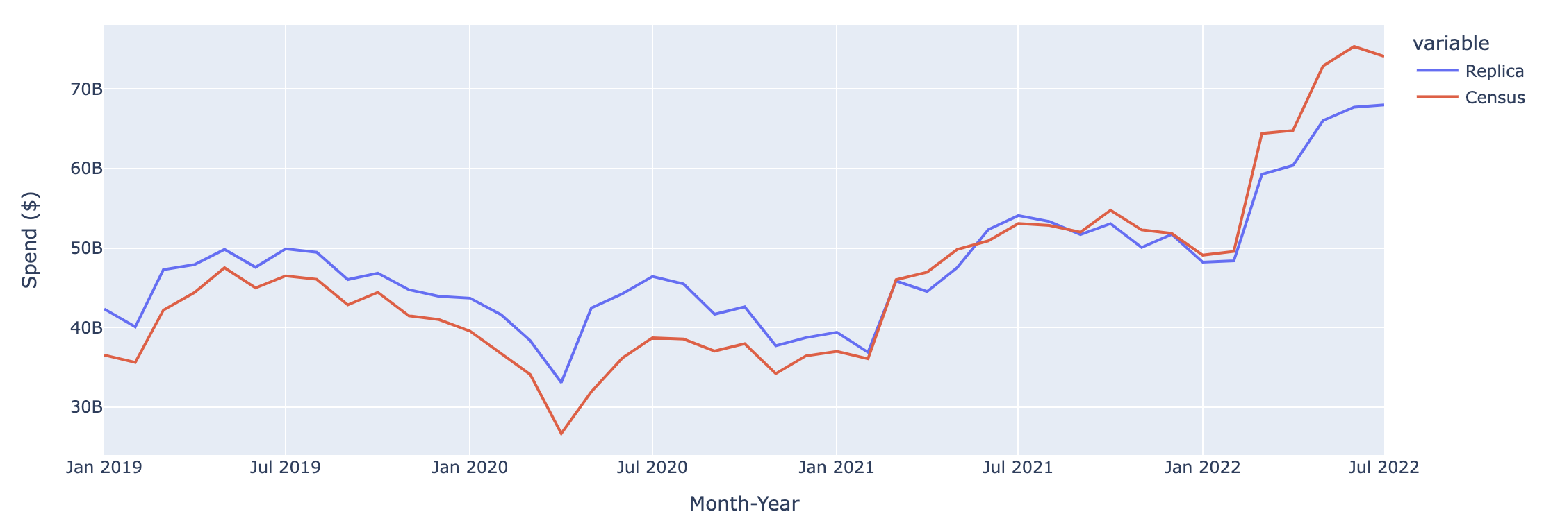
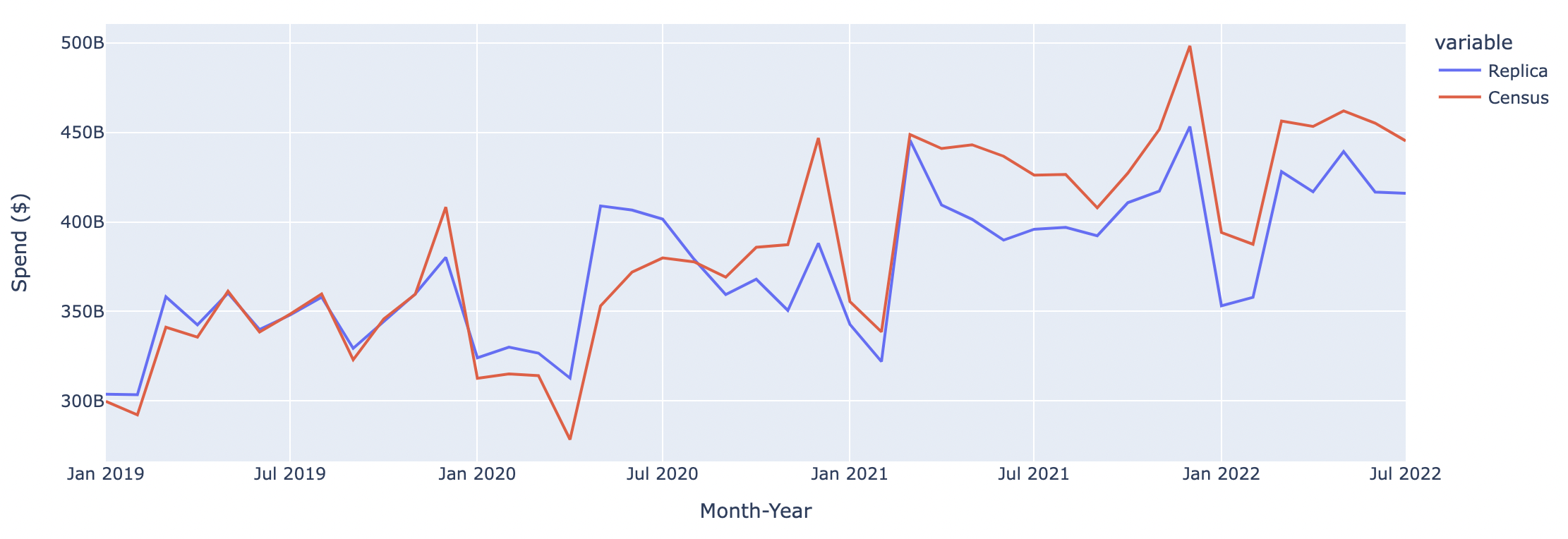
Comparison to US Census Advance Monthly Retail Trade Survey
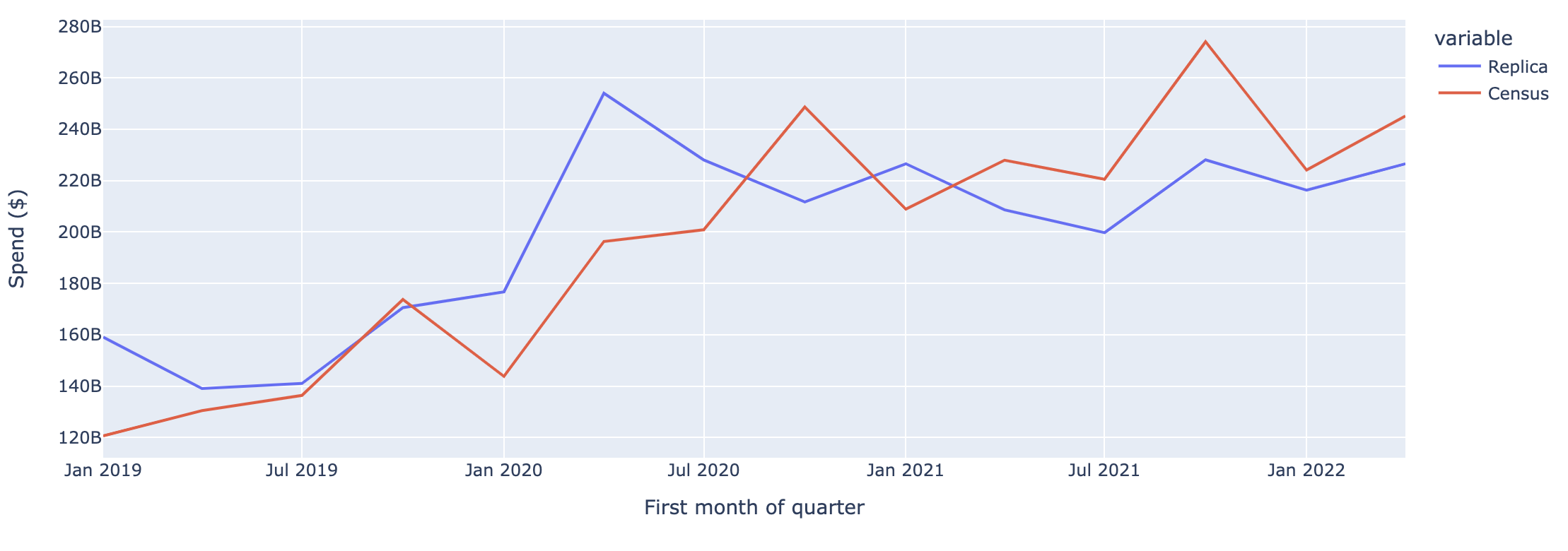
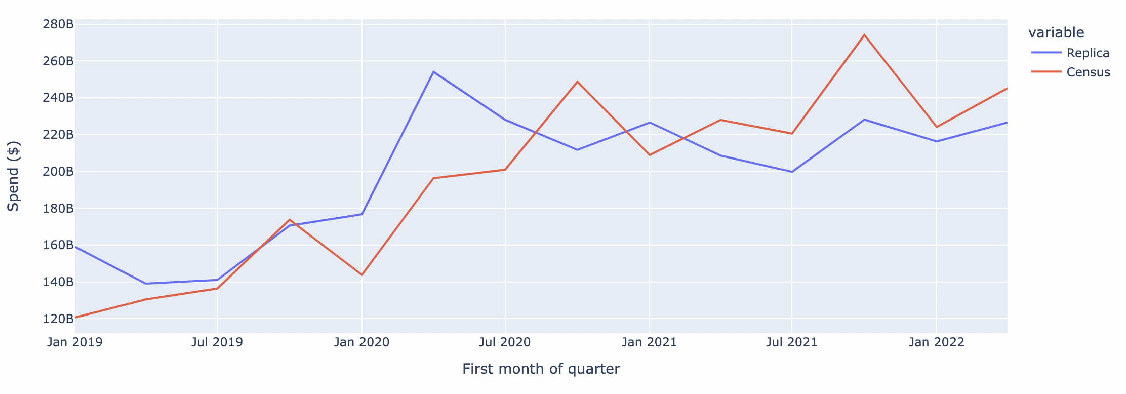
The graphs below compare Replica outputs to Census monthly retail sales data across four spending categories: 1) Grocery Stores, 2) Gas Stations, Parking, Taxis and Tolls, 3) Retail, 4) Restaurants and Bars.
Nationwide Spend at Grocery Stores
Nationwide Spend on Gas Stations, Parking, Taxis, Tolls
Nationwide Spend on Retail
Nationwide Spend at Restaurants and Bars
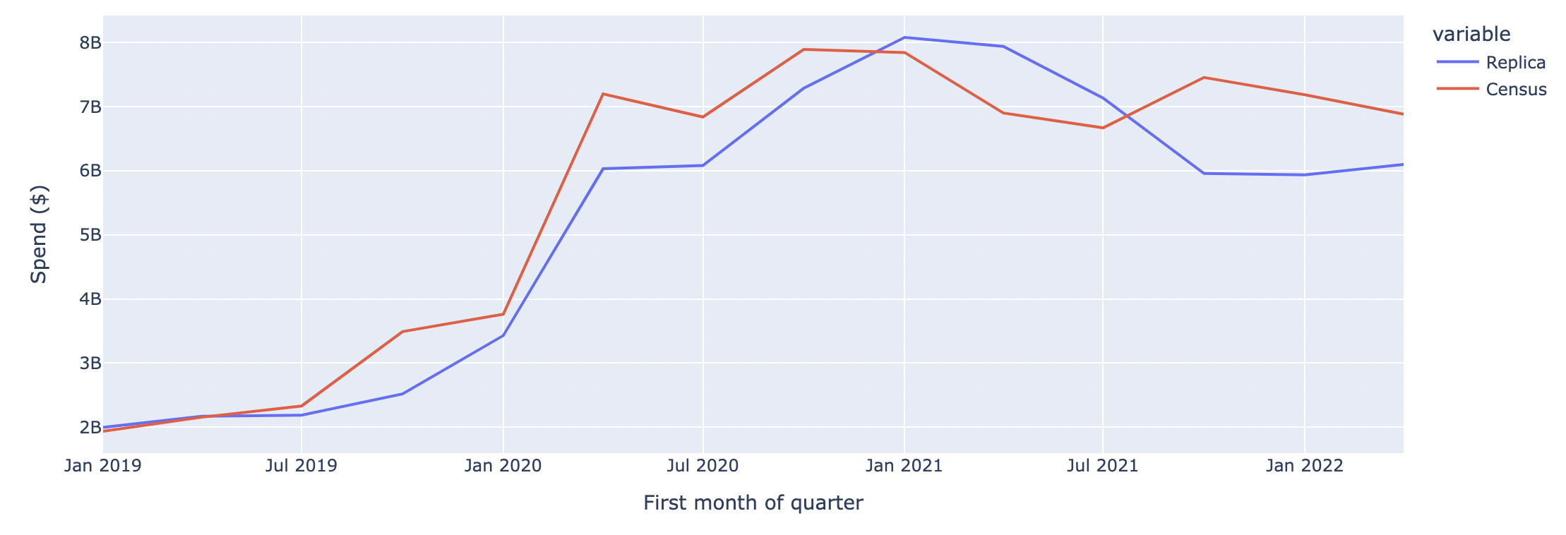
Comparison to US Census Quarterly E-Commerce Report
The graphs below compare Replica outputs to the Census quarterly e-commerce report across two spending categories: 1) Grocery Stores 2) Retail.
Nationwide E-commerce Spend on Grocery Stores
Nationwide E-commerce Spend on Retail
Appendix
Detail about NAICS code granularity
Currently, Replica provides spend data for six industry categories:
- Retail
- Grocery Stores
- Restaurants and Bars
- Gas Stations, Parking, Taxis and Tolls
- Airline, Hospitality, and Car Rental
- Entertainment and Recreation
However, the underlying modeling is performed for finer-grained categories more similar to NAICS-3 codes. The results are then aggregated to create the 6 industry categories above. The underlying modeling is performed for the following categories:
| NAICS | Census | Replica |
|---|---|---|
| 441 | MOTOR_VEHICLES_PARTS | Retail |
| 442 | FURNITURE_STORES | Retail |
| 443 | ELECTRONICS_APPLIANCES | Retail |
| 444 | BUILDING_GARDEN | Retail |
| 445 | GROCERY_STORES | Grocery Stores |
| 446 | PHARMACIES | Retail |
| 447 | GAS_STATIONS | Gas Stations, Parking, Taxis, and Tolls |
| 448 | CLOTHING_STORES | Retail |
| 451 | SPORTING_GOODS | Retail |
| 452 | GENERAL_MERCHANDISE | Retail |
| 453 | MISC_STORE_RETAIL | Retail |
| 454 | NONSTORE_RETAIL | Retail |
| 481 | AIRLINE | Airline, Hospitality, and Car rental |
| 4853 | TAXIS | Gas Stations, Parking, Taxis, and Tolls |
| 5321 | CAR RENTAL | Airline, Hospitality, and Car rental |
| 71 | ENTERTAINMENT_RECREATION | Entertainment and Recreation |
| 721 | HOSPITALITY | Airline, Hospitality, and Car rental |
| 722 | RESTAURANT_BARS | Restaurants and Bars |
| 81293 | PARKING | Gas Stations, Parking, Taxis, and Tolls |
Updated 8 months ago